First-time Users:First-time Users

What is CE-QUAL-W2?

The first step to building a CE-QUAL-W2 model is to understand what CE-QUAL-W2 is. Every definition I've read of the model describes it as a two-dimensional, laterally averaged, hydrodynamic and water-quality model. Let's analyze this definition. Every reservoir has three dimensions. The reservoir width is called the lateral dimension. The reservoir length is called the longitudinal dimension. The third dimension is the vertical dimension, or the reservoir depth. CE-QUAL-W2 is two-dimensional, meaning two of the three dimensions are represented by a series of cells for which governing equations can be solved. The next part of the definition, "laterally averaged," tells us that the two dimensions CE-QUAL-W2 looks at are the longitudinal and vertical dimension. This is why the model is good for long, narrow reservoirs; computations along the length of the reservoir are averaged across the reservoir width. The last part of the model definition refers to the type of computations the model is capable of performing. The model can simulate hydrodynamic behavior (the way water moves) as well as water-quality characteristics.

Define your objectives

Why do you want to build a CE-QUAL-W2 model? Are you concerned with reservoir temperature? Do you want to see how different watershed management practices might affect the water quality of your reservoir? These are questions to think about before you begin building your model. Write down your modeling objective so you have a clear direction as you begin modeling.

Collecting and Gathering Data

This may be the most difficult part of the modeling process, and it doesn't even involve modeling. CE-QUAL-W2 can manage a ton of data. Just take a quick look at the user's manual and you'll see the enormous amounts of data the model is capable of using. In order to identify what data you'll need for your model, refer to your modeling objective. There's a chance someone else has a built a CE-QUAL-W2 model similar to the one you want to build. An entire section on monitoring is available on this wiki that might help you identify what data you need for your particular modeling objective. You'll find it here, or under the monitoring heading on the main page.

Building Input Files

Now that you've identified the data you need, you can start building input files. I suggest starting with the bathymetry file, the control file, and the meteorological file. The bathymetry file describes the geometry of your reservoir. The control file is like an airplane cockpit. It has all the controls and switches that tell CE-QUAL-W2 what files it is looking for, how long to run, what coefficients to use, etc. The meteorological file contains meteorological data, like air temperature, wind speed, wind direction, cloud cover, etc. All three are crucial components of any CE-QUAL-W2 model. Let's discuss how we go about building these files.

Terminology

When referring to the W2 user's manual and other supporting documents, it helps to be familiar with some W2 terminology.

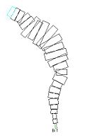
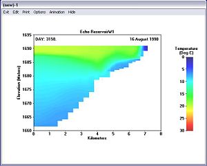
• Segments: These refer to model cells that are arranged in series along the longitudinal axis of your reservoir. Figure 1 is an example of segments created for Echo Reservoir in Summit County, UT.

Echo Reservoir Segment and Layer Profiles

Figure 1. Segments created for Echo Reservoir, UT

Figure 2. Layers created for Echo Reservoir, UT

Figure 3. Layers and Segments

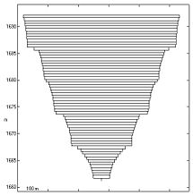
• Layers: These refer to the vertical cells that makeup the vertical layer profile of your model. Echo Reservoir was divided into 0.5 meter layers (Figure 2).

• Branches: Branches are the reason CE-QUAL-W2 is sometimes described as being quasi-three-dimensional. Although the model is laterally averaged, if your reservoir has deep, narrow tributaries coming off the main reservoir, they can be modeled as separate branches, or collections of segments and layers, giving the model a quasi third-dimension. CE-QUAL-W2 has the ability to model separate branches simultaneously, though more branches means significantly more work.

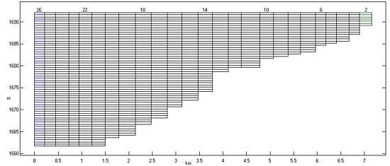
• Dummy Segments: Each branch has two dummy segments at each end. You'll notice in Figure 3, that the segments are numbered 2 through 26. Segments 1 and 27 are dummy segments, required by the model for computational purposes, but not representing any real geometry. You can read more about dummy segments in the user's manual which you'll find on the Portland State website.
  
  

Bathymetry File

The best way I've found to build a bathymetry file is with the Watershed Modeling System, WMS. The processing section provides a good explanation of how WMS can be used to create a bathymetry file. For a step-by-step tutorial on how to build the bathymetry in WMS, click on the link below and find the CE-QUAL-W2 tutorial.

WMS Tutorials

A useful reference for building CE-QUAL-W2 bathymetry files, and the method that is used to determine the bathymetry in WMS, is found on the xmswiki.com web site by clicking here.

Another way you can build your bathymetry, if you don't have a WMS license, is with W2i. The processing section provides a link to the W2i website which explains this utility in more detail. Essentially, the utlity lets you set up a spreadsheet with your reservoir geometry and by clicking "New Build" you can create your bathymetry, control, and other files automatically. I've never used this utility, but it seems to pose a good alternative for modelers who aren't familiar with WMS. Like WMS, you must purchase W2i to use it. Keep in mind that both WMS and AGPM currently only support CE-QUAL-W2 version 3.2.

The Bureau of Reclamation provides helpful dam data that you may want to use when creating your bathymetry. The following link can help you find the dimensions of your dam and helpful hydraulic and hydrologic information.

• Dam Data from the US Bureau of Reclamation
  
  

Control File

The control file is quite complex. In order to build your control file, I would highly recommend starting with an example. Input files for Degray Reservoir are provided along with the legacy W2 models from the Portland State website. You could also use a control file from any working model you have available and start with that. This is where you also want to have the user's manual handy. Using the user's manual, go through the control file and identify what each card (or label) refers to. Change the values to reflect the characteristics of your reservoir. If you're unsure about a value, I'd recommend sticking with the default value suggested by the user's manual.

Check your Bathymetry and Control File

Once you've built your bathymetry and control files, you'll want to check and make sure they are built properly before you go on. The best tool for this is W2i. When you open W2i, click on the "View Bath" button. This will bring up a file browser window in which you'll want to navigate and select your control file (I know, you might think it's weird that you select your control file to check your bathymetry, but like I said, the control file is your cockpit). After selecting your control file, if a window pops up showing images similar to what you see in Figures 1, 2, and 3, then congratulations, your files are built properly. Now you just need to tweak them a little bit to make them a little more accurate. However, there's a good chance this window won't pop up. Instead, you'll get an error and this means there are problems with your bathymetry or control file, or both.

Finding the mistakes in your bathymetry and control files can be a very tedious and time-consuming process if you don't know what to look for. First of all, make sure there are no tabs in your files. Also, check your file layouts. Pay attention to extra lines that may have been inserted at the top of your file. Check the spacing. There are eight spaces allocated for each value and each value should be right justified under the card to which it pertains. After taking all these steps, you may still find that you have errors. Your next debugging step is to use Cole's Pre W2 input checker.

If you haven't yet, download the pre.exe input checker for the model version you are using from the Portland State website. This utility will check all your input files and create a pre.err file indicating what, if any, errors were found. In order to run the utility, however, you must have a complete set of input files in your model folder, whether they are accurate or not. Use the Degray example input files as stand-ins for the files you haven't yet created. You may have to modify the Degray files a bit since I'm pretty sure the Degray model has multiple branches. You may think it's silly to use two files of your own and a dozen files from some other model, but this is honestly the best approach to take. Once you get the model running, you can start replacing files one by one, running the model each time, so that if you get an error, you can easily trace it back to the file that caused it. For now, don't worry about the accuracy of all your input files. Just concentrate on making sure each file shows the right number of JDAYS, and that segment, branch, and waterbody values are consistent with the bathymetry and control files. Once the files look good to you, run pre.exe and check the output file (pre.err), fix any changes, and run it again. Don't expect to fix all your errors all at once, but be patient and sooner or later you'll take care of all your errors.

Meteorological File

The meteorological file contains meteorological data for your reservoir. This includes air temperature, dewpoint temperature, wind speed, wind direction, cloud cover, and solar radiation (which is optional). The user's manual provides lots of helpful information regarding the meteorological file. For now, we'll discuss how you go about getting the data.

There are a couple of approaches you can take to gather meteorological data. What might be the simplest way, is to use W2i (v 3.2). When you open W2i, you'll see a "Find Met" button on the top toolbar. If you click on it, it prompts you to select your control file. The reason it does this is because W2i is going to use the latitude and longitude information in your control file to locate the meteorological stations closest to your reservoir. Select your control file and a window will pop up telling you where the nearest met stations are to your reservoir. In the W2i research version, it appears you can even download the data from these stations within W2i, but I haven't gotten it to work yet. Once this feature gets fully implemented though, this is the way I would recommend doing it for sure. For now, W2i simply helps you identify the stations from which you can obtain met data.

Until W2i's automatic met data retrieval function gets implemented, I suggest downloading your met data from NOAA. The steps below will walk you through this process.

1. Go to the NOAA Climatological Data website
2. Click on the image for "Land Based" data
3. On the Land-based Data page, click "Data and Products"
4. On the Land-based Data and Products page, under Search Methods & Metadata, click the "Search" link
5. Select the type of data you want (Temperature, Wind, Clouds, maybe Solar), select US (or Global for international projects) and the frequency (you'll want hourly). Click Submit.
6. On the Search Results page, select "Integrated Surface Hourly"
7. On the next page, read the NOAA policy and then click "I agree to these terms (continue)"
8. On the next page, click "Continue with ADVANCED Options"
9. On the Surface Data, Hourly Global page, under "Retrieve data for" click "Country" and select your country. Leave the "Select Output Format" as "Text File." Click continue.
10. Select your state and retrieve data for "Selected Stations in the state" and click continue. Again, for international projects this process will be a little different.
11. Now select the station for which you want to retrieve data. You can refer to the list generated by W2i or use your own knowledge of the area to select what you believe to be the closest station. Click continue.
12. On the next page, you'll see a list of all the data elements available for download. For our purposes, we'll select the four cloud related parameters (I can't remember which one you need for cloud cover), Dew Point, Current Temperature, and Wind Direction and Speed. You'll need to hold down the control key to select multiple elements. Click continue.
13. Select the time range for which you need the data, change the output format to "Delimited with station name", leave the Output Format Delimeter to "Comma,", and click continue.
14. Click view inventory to double check your data request. If it looks okay, toggle on that you have viewed the inventory, enter your email address and click Submit Request.
15. You will be sent an email with links to four files (the data may not be available for 24 hours, so you might have to wait overnight before the links will work):
    • Data File: This is the comma separated file containing the data you ordered.
    • Stations included in your search: This text file simply lists the station(s) for which you requested data.
    • Data inventory for your search: This is the inventory file you viewed before submitting your order.
    • Format documentation: This metadata file explains the different columns of data you requested. It's very helpful.
16. Click on each link to view the file in a separate browser window, and click File->Save and rename the file to something more descriptive. I would save all four files even if you think you won't need them.
17. Now simply open up the data in Excel, or your spreadsheet program of choice, and format the data in the way it should appear for your met file (the user's manual has some examples). This sounds easy, but formatting the data can be quite difficult if you aren't familiar with Excel. These tips might help you.
    • To create the JDAY, parse the date and time columns using Excel's "left()" and "right()" functions and combine your separated fields using the "date()" function plus the hour/24 and minute/1440.
    • Set your column widths to 8 to make sure each column in your text file has 8 spaces.
    • Once your data is formatted properly, save your worksheet as a "space delimited (.prn)" file and then once it's saved, you can manually change the extension to .npt which is the extension CE-QUAL-W2 recognizes.
    • If you have several years of data, you may exceed the maximum row number in Excel 2003. In this case, edit your met data in pieces (Open Office Calc - click here for a free download-, lets you import your text file starting from the row just after the max row number in Excel. You might think you can do this in Excel, but I'm pretty sure you can't.)
18. Once you're done editing the met file, go ahead and replace the bogus file you used from the Degray example (if you did so to run the pre W2 checker), and run pre.exe to check for any errors. There's a good chance you will have errors probably related to missing data points. Fix the errors until your pre.exe runs successfully to completion
    
    

You can also find meteorological data at Weather Underground and sometimes through the US Bureau of Reclamation website.

Other Input Files

There are several other input files you'll need to create. They include:

• Daily inflows for each branch
• Temperature inflows for each branch
• Daily inflows from each tributary
• Temperature inflows from each tributary
• Daily outflows from the dam
• Distributed tributary inflow file
• Distributed tributary inflow temperature file
• Shade file
• Graph File
  
  

The Degray example input files are a good guide for building these files.

The following sites may be helpful for finding data. Since every region is different, you'll have to explore a bit to find the best data source for your particular project.

• United States Geological Survey (USGS) Streamflow data
• United States Bureau of Reclamation
• Environmental Protection Agency, STORET
  
  

Calibration

Water Balance

The first thing you want to calibrate is your reservoir volume. First, make sure you have created all inflow and outflow files for your reservoir. The more inflows and outflows you have documented, the easier (and more accurate) will be your water balance. If you haven't already, download the water balance tool from the Portland State website. This tool is used to automatically create a distributed tributary inflow file that balances your water volume. Obviously, you'll need a file indicating the time-varying water surface elevations of your reservoir to guide the water balance iterations. This file simply contains the JDAY and the elevation of the water surface on that day and it's often named el_obs.npt. The document below explains how to go about performing the water balance.

Water Balance Tutorial

The water balance utility also comes with a helpful .pdf document when you download it that further explains its use. You may find that helpful as well.

Temperature

After running your model to completion, you'll likely want to know how accurately your model simulates the actual temperature in the reservoir. The first thing you need to do to prepare for the temperature calibration is to assemble the file containing observed temperature profiles. This file contains five columns: JDAY, KM, ELEV, TEMP, and DATE. JDAY is the model julian day on which the observations were taken, KM refers to the observation location, ELEV is the elevation of each temperature reading, and DATE is the actual date of the observation, entered as MM/DD/YEAR. Like CE-QUAL-W2 input files, this file allocates 8 spaces for each data column. The file extension for this file should be *.dat. For calibration, one profile for each season is usually sufficient.

Once you have assembled your file of observed temperature profiles, the next step is to compare them with your model profiles. AGPM is the most useful tool for viewing your temperature profiles and animations. Unlike the water balance tool, this tool will not perform your temperature calibration for you, but it will help you see how your model temperatures compare with observed temperatures. Again, be aware that AGPM currently only supports CE-QUAL-W2 version 3.2. If you're using AGPM to view your temperature calibration, the following steps will help you get started.

Figure 4. AGPM Temperature Profiles

1. Open AGPM
2. In the "Model Runs" portion of the window, navigate to the folder containing your model runs
3. Select your model folder in the file tree on the left and a *W1 file should appear in the list box to the right
4. Highlight the *W1 file and select Temperature in the constituent list box
5. Click the "Autoprofile" drop down menu and select "Express (Separated)..."
6. In the Get Field Data File window that appears select the *.dat file containing the observed temperature profiles
7. The "Source" window should now list all the temperature profiles that are available for viewing. Select any of the profiles and click "PLOT"
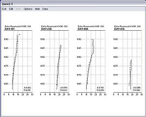
8. Your temperature profiles are all plotted together in a new window. The dotted line is the observed temperature profile and the solid line is the model temperature profile. To view the statistics (AME, RMS) for the plots, click Options->Statistics->This Window. The statistics for will appear in the bottom right hand corner of each plot (Figure 4)
   
   

You can also view temperature animations with AGPM. This isn't incredibly useful for calibration, but it's very useful for presentations and for understanding the behavior of your reservoir over time. It's also really cool. Here's how you do it.

Figure 5. AGPM Temperature Animation

1. Open AGPM
2. In the "Model Runs" portion of the window, navigate to the folder containing your model runs
3. Select your model folder in the file tree on the left and a *W1 file should appear in the list box to the right
4. Highlight the *W1 file and select "Animation" as the plot type
5. In the constituent list box, select "Temperature"
6. Click the "Add Item" button and a new item should appear in the "Source" window
7. Click and highlight the Animation item in the "Source" window and click the "PLOT" button
8. A new window should open up showing the start of a new temperature animation. Start the animation by selecting Animation->Go. This will loop through the temperature output from your model to create a colorful representation of how temperature changes in your reservoir over time
   
   

There are lots of other tools if you want to get into some of the more advanced post-processing, but the ones I've just explained will be the most useful to you.

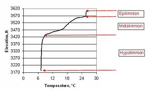
Though there's no tool to perform a quick and easy temperature calibration, there are certain parameters you should pay attention to when trying to calibrate your model for temperature. Diferent parameters will affect the temperature differently in different parts of the water column. Figure 6 shows the three main components of the temperature depth profile. It helps to be familiar with these terms as you work with the temperature calibration.

Figure 6. Zones of Temperature Depth Profile

• Epilimnion: The topmost thermal layer which often exhibits a constant temperature due to evaporation.
• Metalimnion: Often referred to as the thermocline where the temperature is changing rapidly with depth.
• Hypolimnion: The deepest and often the coldest thermal layer where the temperature stops changing with depth. For shallow reservoirs, especially reservoirs where water is released from the bottom of the reservoir, the hypolimnion may not exist.
  
  

To begin, make sure to set all your heat exchange and hydraulic coefficients to their default values (consult the user's manual for default values). Start your calibration by adjusting the following parameters. Make sure to keep a log of what parameter you changed and how it affected your results so you get a feel for how the different parameters change your model as you go along.

• Solar shading (shd.npt): This file controls the percent of solar radiation which actually reaches the water surface. There is a coefficient for each model segment. If your reservoir is in a canyon, the canyon walls may shade your reservoir just after sunrise and just before sunset. You can reflect this behavior in your model by changing the solar shading coefficient. A value of 1.0 results in 100% of the solar radiation reaching the water surface, and a value of 0 means 0% reaches the surface. Solar radiation will affect the overall water column, but changes are most noticeable in the epilimnion. If you need less heat in the epilimnion, you can reduce the shading coefficients. Try not to reduce the coefficients below 0.9 and 0.85 if no other parameter adjustments help.
  
  
• Evaporative wind coefficients AFW, BFW, and CFW (w2_con.npt): For more information on the wind coefficients look up Surface Heat Exchange in appendix A of the user's manual. The wind coefficients are part of an evaporative wind speed function. Increasing the AFW, BFW, and CFW coefficients will increase evaporation. Concentrate first on AFW since it is a linear increase. The other two coefficients are multiplied by the wind speed. The best way to tell whether you need more or less evaporation is to look at the temperature profiles throughout the year, especially in the spring and fall. If the epilimnion is too warm, you need more evaporation to cool the water and vice versa. It may be difficult to determine if you need more or less evaporation since you typically have only a few profiles a year. I suggest waiting until you have tried several other parameters in the calibration before trying this. If you do adjust the evaporation you will need to compare it to estimated evaporation. You will probably need to compare model evaporation to the estimate anyway.
  
  
• Light extinction, EXH2O (w2_con.npt): The light extinction coefficient (EXH2O) is used in calculating the depth to which light can penetrate the water column. The lower the value entered, the further light can penetrate. The default is 0.25 to 0.45. The value for pure water is 0.20. Try testing different values to get a feel for how this value changes temperature results.
  
  
• Sediment temperature, TSED (w2_con.npt): According to the user's manual this value should be set at approximately the average annual air temperature. This is the temperature that will be used in heat exchange calculations for the sediment-water interface. The average annual air temperature should work well. If you notice the hypolimnion is too cold or too warm consistently you may adjust this accordingly.
  
  
• Data input review: Once you have tried everything else and looked over and over at results you may get a feel for what need to be changed. Things such as the air temperature, cloud cover, inflow temperatures, etc. may be fairly obvious. Be mindful of where all the data comes from. Meteorological data often comes from airports that may reside at a higher or lower location than your reservoir.
  
  

Once you have started on the thermal calibration you will want to know how much time you should spend on it. I suggest the following goals: try for an AME of less than 1 deg C. An AME of around 0.5 deg C would be fantastic. You could probably continue in the thermal calibration for some time but at some point enough is enough. You will reach the point where the model will serve its intended purposes although it may not be exact.